17 KiB
| created_at | title | url | author | points | story_text | comment_text | num_comments | story_id | story_title | story_url | parent_id | created_at_i | _tags | objectID | year | |||
|---|---|---|---|---|---|---|---|---|---|---|---|---|---|---|---|---|---|---|
| 2015-11-03T10:10:23.000Z | Cosines and correlation (2010) | http://www.johndcook.com/blog/2010/06/17/covariance-and-law-of-cosines/ | ColinWright | 49 | 17 | 1446545423 |
|
10498549 | 2010 |
Cosines and correlation
![]()
(832) 422-8646
Cosines and correlation
Posted on 17 June 2010 by John
Preview
This post will explain a connection between probability and geometry. Standard deviations for independent random variables add according to the Pythagorean theorem. Standard deviations for correlated random variables add like the law of cosines. This is because correlation is a cosine.
Independent variables
First, let’s start with two independent random variables X and Y. Then the standard deviations of X and Y add like sides of a right triangle.
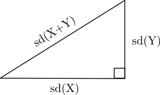
In the diagram above, “sd” stands for standard deviation, the square root of variance. The diagram is correct because the formula
Var(X+Y) = Var(X) + Var(Y)
is analogous to the Pythagorean theorem
_c_2 = _a_2 + _b_2.
Dependent variables
Next we drop the assumption of independence. If X and Y are correlated, the variance formula is analogous to the law of cosines.
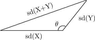
The generalization of the previous variance formula to allow for dependent variables is
Var(X+Y) = Var(X) + Var(Y) + 2 Cov(X, Y).
Here Cov(X,Y) is the covariance of X and Y. The analogous law of cosines is
_c_2 = _a_2 + _b_2 – 2 a b cos(θ).
If we let a, b, and c be the standard deviations of X, Y, and X+Y respectively, then cos(θ) = -ρ where ρ is the correlation between X and Y defined by
ρ(X, Y) = Cov(X, Y) / sd(X) sd(Y).
When θ is π/2 (i.e. 90°) the random variables are independent. When θ is larger, the variables are positively correlated. When θ is smaller, the variables are negatively correlated. Said another way, as θ increases from 0 to π (i.e. 180°), the correlation increases from -1 to 1.
The analogy above is a little awkward, however, because of the minus sign. Let’s rephrase it in terms of the supplementary angle φ = π – θ. Slide the line representing the standard deviation of Y over to the left end of the horizontal line representing the standard deviation of X.
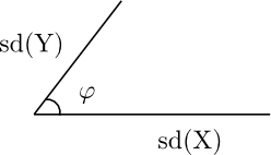
Now cos(φ) = ρ = correlation(X, Y).
When φ is small, the two line segments are pointing in nearly the same direction and the random variables are highly positively correlated. If φ is large, near π, the two line segments are pointing in nearly opposite directions and the random variables are highly negatively correlated.
Connection explained
Now let’s see the source of the connection between correlation and the law of cosines. Suppose X and Y have mean 0. Think of X and Y as members of an inner product space where the inner product <X, Y> is E(XY). Then
<X+Y, X+Y> = < X, X> + < Y, Y> + 2<X, Y >.
In an inner product space,
<X, Y > = || X || || Y || cos φ
where the norm || X || of a vector is the square root of the vector’s inner product with itself. The above equation defines the angle φ between two vectors. You could justify this definition by seeing that it agrees with ordinary plane geometry in the plane containing the three vectors X, Y, and X+Y.
For daily posts on probability, follow @ProbFact on Twitter.

Categories : Math Statistics
Tags : Math Probability and Statistics
Bookmark the permalink
Post navigation
Previous PostWhy computers have two zeros: +0 and -0
Next PostPorting Python to C#
19 thoughts on “Cosines and correlation”
Nice write-up. I sneak this into my lectures occasionally to perk up the math majors, who don’t always notice the many interesting mathematical objects that appear in statistics. ( The denominator for correlation, sd(X)sd(Y), is the geometric mean of the two variances–what’s THAT all about, guys? )
Nice! It would only take a current events example to make a cool enrichment activity. Thank you!
- Ger Hobbelt
Thank you for this; showing up right when I needed it! Alas, it would have been extra great if my teachers had pointed out this little bit of intel about 25 years ago, while they got me loathing those ever-resurfacing bloody dice even more. Meanwhile, I’ve shown to be dumb enough not to recognize this ‘correlation’ with lovely goniometrics on my own.
Despite all that I’ve found the increasing need for understanding statistics (as you work on/with statistical classifiers and you feel the need to really ‘get’ those s.o.b.s for only then do you have a chance at reasoning why they fail on you the way they do) and your piece just made a bit of my brain drop a quarter — I’m Dutch; comprehension is so precious around here we are willing to part with a quarter instead of only a penny 😉
-
Pingback: Relación entre la ley de cosenos y correlación de variables « Bitácoras en Estadística
-
Harry Hendon
Hi John, maybe you can help on a related problem, which I think uses the law of cosines as well (but I lost my derivation):
If you know the two correlations of one time series with two other predictor time series, what does this tell you about the possible range of correlation between the two predictor time series. That is, given r(X,Y)=a and r(X,Z)=b, what is the possible range of r(Y,Z)=c in terms of a and b?
Of course some examples are intuitively trivial (eg, if a=b=1, then c=1, and if a=0 but b=1 then c=0). But, consider if a=b=.7 (which are strong correlations), then I think the possible range of c is still enormous (0.<c<1. ). In this case, I reasoned because X accounts for half the variance of Z and Y accounts for half the variance of Z that X could possibly account for the same half of the variance as Y (ie c=r(X,Y)=1). Or, X could account completely for the other half of the variance that is not accounted for by Y but together X and Y account for all of the variance of Z (ie c=r(X,Y)=0). This understanding has, for instance, implications for (over) interpreting causality based on empirical evidence.
nice article John. We’re looking for more of this.
-
Pingback: Mathematics and Multimedia Blog Carnival #1 « Mathematics and Multimedia
-
Peter Urbani
Hi John -nice post. If you google “four moment risk decomposition” “urbani” you will find a spreadsheet and a presentation illustrating a related problem in risk that you may be interested in or able to help with.
In that method we step backwards through the Cornish Fisher Expansion to the normal distribution to arrive at the vector length or penalty function used Value at Risk calculations but allowing to solve for the higher moments of skewness and kurtosis also. In risk these can be thought of as additional positive or negative risk penalty vectors but ones which interact with each other. The difficulty here is that in the multivariate setting the interaction embeds the weighting as well where we would ideally like a weight independent solution.
In essence we are treating the skewness as an additional positive or negative vector length and the kurtosis as a change in angle. We cheat by Woking backwards from the univariate solution but have to recalculate the modified correlation matrix each time the weights change which is very computationally expensive. I wonder if you can think of a more elegant global satisfying solution ?
May not be possible since we are essentially trying to reduce a 4dim problem to a 2dim one.
People who like this connection between statistics and geometry should read
The Geometry of Multivariate Statistics by Thomas D. Wickens. It is extremely readable and it shows the connection between statistical concepts and the basic geometry of vector spaces.
As the rare individual who loves both Geometry AND Statistics, this is one of my favorite relationships I share with my students. Thanks for the great write up!
@Rick, thanks for sharing… I will definitely have to read that!
- Mudasiru Sefiu
Nice write up, more power on your elbow.
- Michael
What is the geometric interpretation of the requirement that X and Y have zero means? It’s clear that / || X || || Y || != ρ if this assumption doesn’t hold.
- Michael
Oops, it looks like the comment engine mistook my angled brackets for HTML; I was trying to re-write the formula under “inner product space” after solving for cos(theta): X · Y / ||X|| ||Y||
I’ve always wondered whether there is a connection between the angle between the lines of regression of y on x and x on y and the correlation between x and y. Is it as simple cos(theta)? Certainly if r=0, the angle is 90 and cos(90)=0. Similarly if r=1, theta=0 and cos(0)=1.
Is it possible to use this argument to demonstrate why discrete cosine transforms are suitable for data compression?
- klo
What a simple analogy! Thanks for this revelation
Cheers to @Ger Hobbelt, with whom I share exact experience, only that I took the exam 2 year ago, and I hated it and all those examples with dices and colored balls. Sheesh
-
Pingback: Expected value estimates you can take (somewhat) literally - The Polemical MedicThe Polemical Medic
-
sandy
Its 6am here in FL. I have a math certification test later this morning, and I couldn’t sleep b/c the relationship you describe in your post occurred to me while lying in bed; I had to get up and google “cosine and correlation” and up came your post!
Peter Urbani’s comment above asked about a more elegant solution when moving to the multivariate world and recalculating the correlation matrix…he expressed some doubt that the idea could be extended to the multivariate realm: “May not be possible since we are essentially trying to reduce a 4dim problem to a 2dim one.”
Fermat’s Theorem popped into my head when I saw this…got me thinking maybe there is a more elegant proof to this Theorem than what Andrew Wiles was able to produce? Showing why Mr Urbani’s suspicions are correct might be essentially proving Fermat’s Last Theorem?
Anyway, glad I found your post! Do you have any advice for an aspiring Actuary?
Leave a Reply Cancel reply
Your email address will not be published. Required fields are marked *
Comment
Notify me of followup comments via e-mail
Name *
Email *
Website
Search for:

John D. Cook, PhD
Latest Posts
- Fibonacci / Binomial coefficient identity
- Painless project management
- New animation feature for exponential sums
- Quantifying normal approximation accuracy
- Ordinary Potential Polynomials
Categories
CategoriesSelect CategoryBusinessClinical trialsComputingCreativityGraphicsMachine learningMathMusicPowerShellPythonScienceSoftware developmentStatisticsTypographyUncategorized
| ----- |
|  | Subscribe via email |
|
| Subscribe via email |
|  | Subscribe via RSS |
|
| Subscribe via RSS |
|  | Monthly newsletter |
John D. Cook
© All rights reserved.
Search for: