hn-classics/_stories/2008/15763308.md

created_at	title	url	author	points	story_text	comment_text	num_comments	story_id	story_title	story_url	parent_id	created_at_i	_tags	objectID	year
2017-11-23T06:52:13.000Z	A logarithmic image transformation (2008)	http://www.josleys.com/article_show.php?id=82	aekt	87			4					1511419933	story author_aekt story_15763308	15763308	2008

Source

The mathematics behind the Droste effect. This article uses jsMath which requires Java.

| ----- |

| | | |

|

| Home | Galleries | Articles | References | Forum | Links | About |

| | |

|

The mathematics behind the Droste effect.

This article uses jsMath which requires Java.

Posted on 2008-12-26 21:20 | | |

A logarithmic image transformation

Jos Leys

**Abstract: **_An image transformation method, first used by the artist M.C. Escher, and described by Lenstra et al. is generalized for use in a graphics program. _

|
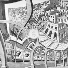
Figure 1: Escher's "Printgallery"[1]10 |

In 1956, Maurits Cornelis Escher completed a drawing called Print Gallery. The drawing depicts a young man looking at a print in a gallery that is deformed almost beyond recognition. There is an enigmatic white area in the center of the image.

In 2003, a group of mathematicians at Leiden University, led by Prof. Hendrik Lenstra succeeded in unraveling the mathematical structure of the image.[2]11 Once this structure was known, they could complete the image by filling in the famous white spot with the help of a computer algorithm.

A summary of their method was published in a paper [3]12 , and received a lot of acclaim, not only in academic circles, but also in the general press.

|

In this article I will show how Lenstras method can be applied more generally for the transformation of images, and the generation of endless zoom animations.

The transformation consists of three stages, which will be described hereunder:

Stage 1: transformation by log(z). ( base e logarithm).

The transformation z mapsto log(z) will transform the complex plane in a strip running from -infty to +infty along the real axis with a width equal to 2$pi$: any point on the complex plane can be represented as re^{itheta}, so log(z)=log(r)+itheta. As 0leqthetaleq2pi,all points will be transformed to a strip of width 2pi.

However as re^{itheta}=re^{i(theta+n2pi)} for any integer n, any parallel strip between n2pi and (n+1)2pi can be considered as an image of the complex plane: in other words, log(z) will transform the complex plane into an infinite number of copies..

For our image transformation, lets consider how log(z) transforms the area between a set of concentric circles of radius r_1 and r_2. ( Fig. 2).

| ----- | |
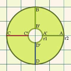
Figure 2: Concentric circles. | |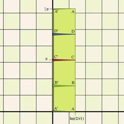
Figure 3: Circles transformed by log(z). |

The transformation illustrated in Figs. 2 and 3 is the transformation zmapsto log(frac{z}{r_1}) . The outer circle becomes a vertical line at$log(frac{r_2}{r_1})$ , and the inner circle is transformed to a vertical line at zero: we have cut the disc of Fig. 1 along line A-A, and bent it into a rectangle.

Stage 2: Rotation and scaling.

The rectangle in Fig.3 is now rotated so that its diagonal coincides with the imaginary axis, and the rectangle is shrunk so that the diagonal is equal to 2$pi$. In transformation terms, this is equal to zmapsto zfe^{ialpha}, with alpha=arctan(frac{log(r_2/r_1}{2pi}) and f=cos(alpha) . (Fig. 4)

| ----- | |
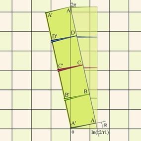
Figure 4: rotation and scaling |

In the next stage we will do the transformation that is the inverse of the log transformation of phase 1.

Stage 3: exponentiation.

We will now transform the rectangle of Fig.4 with the transformation zmapsto e^z . This produces the image in Fig. 5:

All the sides of the rectangle of Fig. 4 are transformed into spirals. Notice that points A and A now coincide, as they were transformed from 2pi i and 0 respectively, which both transform to 1.

| ----- | |
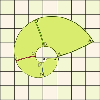
Figure 5: Exponential transformation. |

This concludes the basic transform.

Combining all the stages, the transformation becomes $$zmapsto (frac{z}{r_1})^beta,$$ where beta=fe^{ialpha}. The original image of two concentric circles will be transformed into an identical image by the transformation zmapsto frac{z}{r_2/r_1}, so for the transformed image, an identical copy is obtained if z is divided by (frac{r_2}{r_1})^beta .This means a scaling by |(frac{r_2}{r_1})^beta| and a rotation by minus the argument of$(frac{r_2}{r_1})^beta$.

We now go back to stage 2. We replicate the rectangle of Fig. 4 so that it tiles the plane, and then do the stage 3 transformation again.

| ----- | |
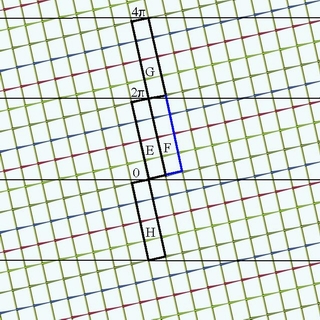
Figure 6: Tiling | |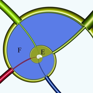
Figure 7: Exponentiation of the tiling |

Rectangle E in Fig. 6 is the original rectangle of Fig. 5, and is transformed by stage 3 to the area E in Fig. 7. Rectangle G and H will also be transformed to area E. Rectangle F will be transformed to area F in Fig. 7. We thus obtain an infinite number of replicas of the original image, transformed so that they tile in spiral form in a seamless fashion. All the replicas are self-similar: area E in Fig.7 can be enlarged and rotated to cover area F exactly.

The configuration of stage 2, where the rectangle is rotated and scaled so that the diagonal is vertical, and equals 2$pi$ is not the only one possible. All possible configurations are shown in Fig.8. If the rotation is 0 or 180 and the scaling factor equals 1, the transformation will produce an infinite number of concentric copies of the original image. In all other cases, the scaling equals f=cos(alpha) ,and the rotation equals$alpha$ , pi-alpha, pi+alpha, or -alpha.

| ----- | |
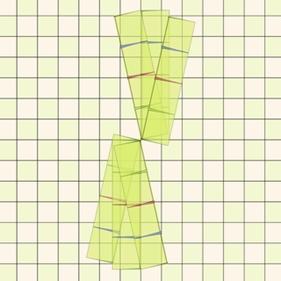
Figure 8: Possible configurations |

In summary, the transformation logic is as follows:

• Choose r_1 and r_2 ( a slight adaptation is necessary to allow circle centers different from the origin).
• Calculate alpha, f, and beta .
• Calculate beta log(z/r_1) for the area between the circles, tile the resulting rectangle, and finally calculate$e^{beta log(z/r_1)}$ for all pixels.

The transformation was implemented in Ultrafractal [4]12, a graphics program that features user defined algorithms, and some examples follow below:

| ----- | |
Figure 9: image 1, original |
Figure 10: image 1, transformed |
|
Figure 11: image 2, original |
Figure 12: image 2, transformed |
|
Figure 13: image 3, original |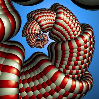
Figure 14: image 3, transformed |

The algorithm can be adapted to allow for non-concentric circles, or even non-concentric polygons.
The area between the two squares in Fig. 15a is transformed by the log transformation into the shaded area in Fig. 15b. This area is then tiled taking into account the angle offset between the two squares. After exponentiation, Fig. 15c is obtained. With a rotation of the tiling after the log transformation, the outcome is Fig. 15d.

| ----- | |
Figure 15a |
Figure 15b |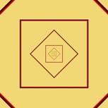
Figure 15c |
Figure 15d |

One can zoom in or out on the transformed images indefinitely. The value of beta can be calculated from the size ratio of the small image vs. the large, and this allows to calculate the magnification and rotation needed to obtain an image that is identical to the start image. A limited number of frames thus suffices to obtain and endless zoom movie, provided the video file is shown in loop mode. Fig.16 shows such a zoom movie. ( A Droste effect movie)

-----
Figure 16

Fig.17 shows anarrangement whereby the smaller square is off-center versus the large square. We now need to calculate the fixed point of the transformation. With C_L =center of large square, $C_S$=center of small square, theta = offset angle between the two squares and m = ratio of the side of the small square vs. the large square, the fixed point C_F is given by:

C_F=C_L+frac{(C_L-C_S)}{(1-me^{itheta})}

The log transform then takes the form zmapsto log( frac{(z-C_F)}{a}) with a = the shortest distance from C_F to the edge of the small square.
The overall transform becomes zmapsto (frac{(z-C_F)}{a})^beta, where beta=fe^{ialpha}, with f=frac{2pi}{(2pi-theta)}cos(alpha), alpha=arctan(frac{ln(m)}{2pi}) .
An identical copy is achieved through a scaling and rotation by the absolute value and the argument of Large m^{frac{fe^{i(alpha-phi)}}{cos(phi)}} with phi=arctan(frac{theta}{log(m)}).

| ----- | |
Figure 17a |
Figure 17b |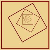
Figure 17c |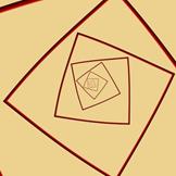
Figure 17d |

The figures below show some examples.

| ----- | |
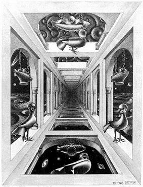
Figure 19: LW346 by M.C. Escher[1]10 |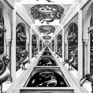
Figure 20: Transformed image |
|
Figure 21: Original |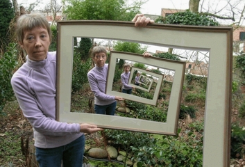
Figure 22: Transformed |

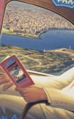
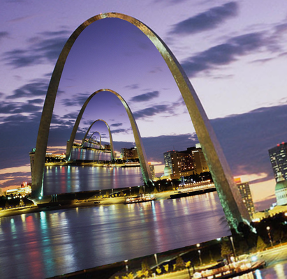
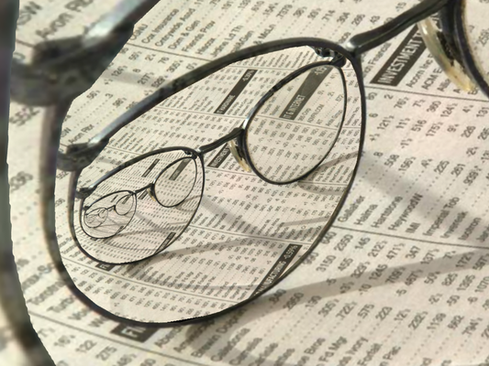
Fig. 23 shows frames from a Droste effect animation based on a vintage airline poster.

| ----- | | | | | | | |
| Figure 23 | | | | | |

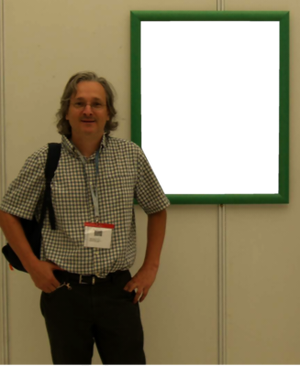
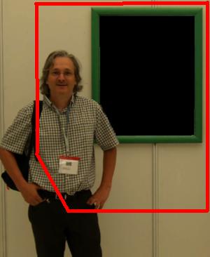
Finally, the transformation can also be applied to any shape. In this case, the shape in question has to be made fully transparent. One can then have the algorithm find the rim of the shape byreading the alpha channel of the image file. The alpha channel value for a transparent pixel is zero, so a simple algorithm can find the location of the rim. Figure 24 shows a sequence of images to illustrate this: The area in the picture on the wall in the image on the right is first made transparent, as to obtain the middle image. One then chooses a point in the transparent area, and a size factor. This will then create a similar area outside the transparent area (which may be rotated versus the transparent image)., as in the image on the right.

| ----- | | | | |
| Figure 24 | | |

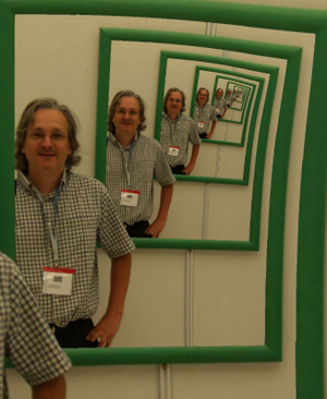
This can then create the following images:

| ----- | | | | |
| Figure 25 | | |

Below are some other examples of free-form image shapes.

| ----- | | | |
| Figure 26 | |

Professor Lenstra and his team proved that the M.C. Escher Print Gallery image has a ratio m=frac{r_2}{r_1}=256 . This means that the rotation angle for stage 2 is alpha=arctan(frac{log(r_2/r_1}{2pi}) or 41.429..degrees, and the scale factor f=cos(alpha) or 0.749767 . .
With beta=fe^{ialpha}, |(frac{r_2}{r_1})^beta| = 22.5836, and the argument of$|(frac{r_2}{r_1})^beta|$ is 157.62559degrees, so an identical image is obtained by zooming by a factor of 22.5836and a rotation by -157.62559degrees.

It is amazing that M.C. Escher drew his Print Gallery by intuition, as he was untrained in mathematics.[5]52 Yet, his image is very close to the computer generated image, based on the above algorithm. It is also known that Escher spent a very long time on this drawing. It makes one wonder what he could have done with a computer.

References

1 2006 The M.C. Escher Company, the Netherlands. All rights reserved. Used by permission.

2 Escher and the Droste effect. http://escherdroste.math.leidenuniv.nl/.

3 B. de Smit and H. W. Lenstra Jr: The mathematical structure of Eschers Print Gallery. Notices of the AMS, Volume 50, number 4.

4 Ultrafractal by Frederik Slijkerman

5 The MacTutor History of Mathematics archive. (webpage)

---

Back to articles index

| | |
Copyright 2018 Jos Leys |

| | | |